Spherical harmonic comparisons

Comparing analytical spherical harmonic solutions to PFSS output.

First, import required modules

import astropy.units as u
import matplotlib.pyplot as plt
import numpy as np
import sunpy.map
from matplotlib.gridspec import GridSpec

import pfsspy
from pfsspy import analytic

Setup some useful functions for testing

def theta_phi(nphi, ns):
    # Return a theta, phi grid with a given numer of points
    phi = np.linspace(0, 2 * np.pi, nphi)
    s = np.linspace(-1, 1, ns)
    s, phi = np.meshgrid(s, phi)
    theta = np.arccos(s)
    return theta * u.rad, phi * u.rad


def brss_pfsspy(nphi, ns, nrho, rss, l, m):
    # Return the pfsspy solution for given input parameters
    theta, phi = theta_phi(nphi, ns)

    br_in = analytic.Br(l, m, rss)(1, theta, phi)

    header = pfsspy.utils.carr_cea_wcs_header('2020-1-1', br_in.shape)
    input_map = sunpy.map.Map((br_in.T, header))

    pfss_input = pfsspy.Input(input_map, nrho, rss)
    pfss_output = pfsspy.pfss(pfss_input)
    return pfss_output.bc[0][:, :, -1].T


def brss_analytic(nphi, ns, rss, l, m):
    # Return the analytic solution for given input parameters
    theta, phi = theta_phi(nphi, ns)
    return analytic.Br(l, m, rss)(rss, theta, phi).T

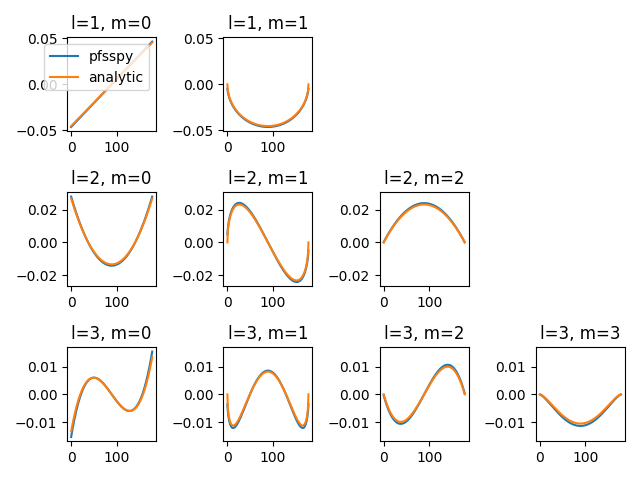
Compare the the pfsspy solution to the analytic solutions. Cuts are taken on the source surface at a constant phi value to do a 1D comparison.

ls = [1, 2, 3]
fig = plt.figure(tight_layout=True)
gs = GridSpec(len(ls), len(ls) + 1)


for i, l in enumerate(ls):
    ax0 = fig.add_subplot(gs[i, 0])
    axs = [fig.add_subplot(gs[i, j], sharey=ax0) for j in range(1, l + 1)]
    axs = [ax0] + axs
    for j, m in enumerate(list(range(l + 1))):
        ax = axs[j]
        nphi = 359
        ns = 179
        rss = 2.5
        nrho = 20

        br_pfsspy = brss_pfsspy(nphi, ns, nrho, rss, l, m)
        br_actual = brss_analytic(nphi, ns, rss, l, m)

        ax.plot(br_pfsspy[:, 180], label='pfsspy')
        ax.plot(br_actual[:, 180], label='analytic')
        ax.set_title(f'l={l}, m={m}')
        if i == 0 and j == 0:
            ax.legend()

plt.show()