Note
Click here to download the full example code
Overplotting field lines on AIA maps
This example shows how to take a PFSS solution, trace some field lines, and overplot the traced field lines on an AIA 193 map.
First, we import the required modules
import os

import astropy.units as u
import matplotlib.pyplot as plt
import numpy as np
import sunpy.io.fits
import sunpy.map
from astropy.coordinates import SkyCoord

import pfsspy
import pfsspy.tracing as tracing
from pfsspy.sample_data import get_gong_map
Load a GONG magnetic field map
gong_fname = get_gong_map()
gong_map = sunpy.map.Map(gong_fname)
Load the corresponding AIA 193 map
if not os.path.exists('aia_map.fits'):
    import urllib.request
    urllib.request.urlretrieve(
        'http://jsoc2.stanford.edu/data/aia/synoptic/2020/09/01/H1300/AIA20200901_1300_0193.fits',
        'aia_map.fits')

aia = sunpy.map.Map('aia_map.fits')
dtime = aia.date
The PFSS solution is calculated on a regular 3D grid in (phi, s, rho), where rho = ln(r), and r is the standard spherical radial coordinate. We need to define the number of grid points in rho, and the source surface radius.
nrho = 25
rss = 2.5
From the boundary condition, number of radial grid points, and source
surface, we now construct an Input object that stores this information
pfss_in = pfsspy.Input(gong_map, nrho, rss)
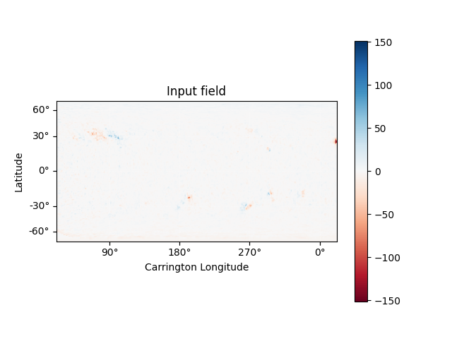
Using the Input object, plot the input photospheric magnetic field
m = pfss_in.map
fig = plt.figure()
ax = plt.subplot(projection=m)
m.plot()
plt.colorbar()
ax.set_title('Input field')
Out:
INFO: Missing metadata for solar radius: assuming the standard radius of the photosphere. [sunpy.map.mapbase]
INFO: Missing metadata for solar radius: assuming the standard radius of the photosphere. [sunpy.map.mapbase]

Text(0.5, 1.0, 'Input field')
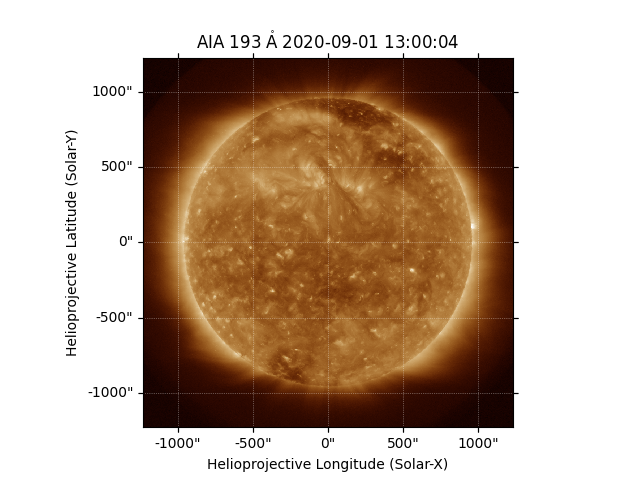
We can also plot the AIA map to give an idea of the global picture. There is a nice active region in the top right of the AIA plot, that can also be seen in the top left of the photospheric field plot above.
ax = plt.subplot(1, 1, 1, projection=aia)
aia.plot(ax)
Out:
<matplotlib.image.AxesImage object at 0x7f5d984dca50>
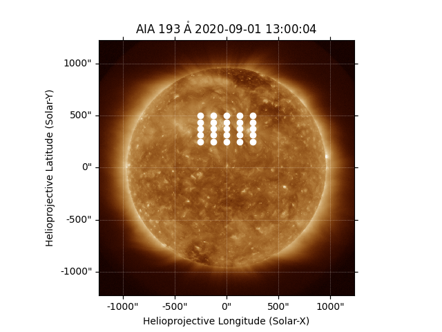
Now we construct a 5 x 5 grid of footpoitns to trace some magnetic field lines from. These coordinates are defined in the helioprojective frame of the AIA image
hp_lon = np.linspace(-250, 250, 5) * u.arcsec
hp_lat = np.linspace(250, 500, 5) * u.arcsec
# Make a 2D grid from these 1D points
lon, lat = np.meshgrid(hp_lon, hp_lat)
seeds = SkyCoord(lon.ravel(), lat.ravel(),
                 frame=aia.coordinate_frame)
fig = plt.figure()
ax = plt.subplot(projection=aia)
aia.plot(axes=ax)
ax.plot_coord(seeds, color='white', marker='o', linewidth=0)
Out:
[<matplotlib.lines.Line2D object at 0x7f5da26dd110>]
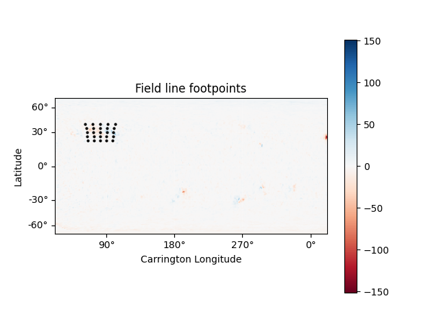
Plot the magnetogram and the seed footpoints The footpoints are centered around the active region metnioned above.
m = pfss_in.map
fig = plt.figure()
ax = plt.subplot(projection=m)
m.plot()
plt.colorbar()

ax.plot_coord(seeds, color='black', marker='o', linewidth=0, markersize=2)

# Set the axes limits. These limits have to be in pixel values
# ax.set_xlim(0, 180)
# ax.set_ylim(45, 135)
ax.set_title('Field line footpoints')
ax.set_ylim(bottom=0)
Out:
(0.0, 179.5)
Compute the PFSS solution from the GONG magnetic field input
pfss_out = pfsspy.pfss(pfss_in)
Trace field lines from the footpoints defined above.
tracer = tracing.FortranTracer()
flines = tracer.trace(seeds, pfss_out)
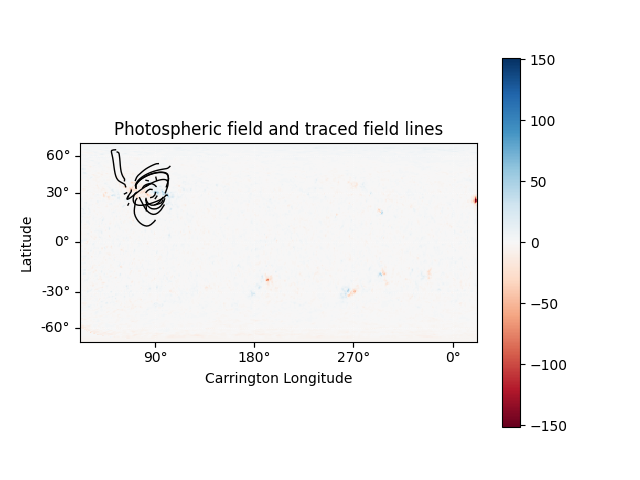
Plot the input GONG magnetic field map, along with the traced mangetic field lines.
m = pfss_in.map
fig = plt.figure()
ax = plt.subplot(projection=m)
m.plot()
plt.colorbar()

for fline in flines:
    ax.plot_coord(fline.coords, color='black', linewidth=1)

# Set the axes limits. These limits have to be in pixel values
# ax.set_xlim(0, 180)
# ax.set_ylim(45, 135)
ax.set_title('Photospheric field and traced field lines')
Out:
Text(0.5, 1.0, 'Photospheric field and traced field lines')
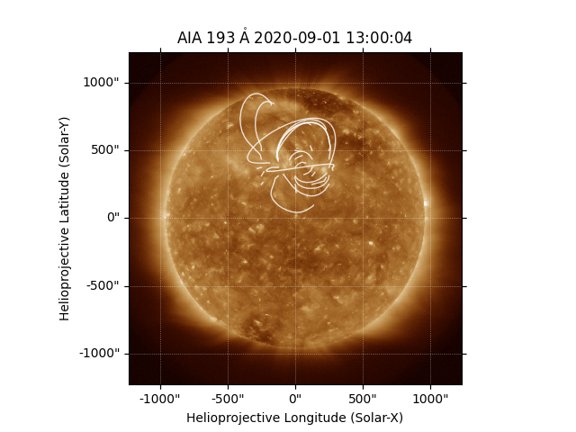
Plot the AIA map, along with the traced magnetic field lines. Inside the loop the field lines are converted to the AIA observer coordinate frame, and then plotted on top of the map.
fig = plt.figure()
ax = plt.subplot(1, 1, 1, projection=aia)
aia.plot(ax)
for fline in flines:
    ax.plot_coord(fline.coords, alpha=0.8, linewidth=1, color='white')

# ax.set_xlim(500, 900)
# ax.set_ylim(400, 800)
plt.show()

# sphinx_gallery_thumbnail_number = 5
Total running time of the script: ( 0 minutes 8.099 seconds)