HMI PFSS solutions

Calculating a PFSS solution from a HMI synoptic map.

This example shows how to calcualte a PFSS solution from a HMI synoptic map. There are a couple of important things that this example shows:

• HMI maps have non-standard metadata, so this needs to be fixed

• HMI synoptic maps are very big (1440 x 3600), so need to be downsampled in order to calculate the PFSS solution in a reasonable time.

import os

import astropy.units as u
import matplotlib.pyplot as plt
import sunpy.map
from sunpy.net import Fido
from sunpy.net import attrs as a

import pfsspy
import pfsspy.utils

Set up the search.

Note that for SunPy versions earlier than 2.0, a time attribute is needed to do the search, even if (in this case) it isn’t used, as the synoptic maps are labelled by Carrington rotation number instead of time

time = a.Time('2010/01/01', '2010/01/01')
series = a.jsoc.Series('hmi.synoptic_mr_polfil_720s')
crot = a.jsoc.PrimeKey('CAR_ROT', 2210)

Do the search.

If you use this code, please replace this email address with your own one, registered here: http://jsoc.stanford.edu/ajax/register_email.html

result = Fido.search(time, series, crot,
                     a.jsoc.Notify(os.environ["JSOC_EMAIL"]))
files = Fido.fetch(result)

Out:

Export request pending. [id=JSOC_20220225_310_X_IN, status=2]
Waiting for 0 seconds...
INFO: max_splits keyword was passed and set to 1. [sunpy.net.jsoc.jsoc]
1 URLs found for download. Full request totalling 6MB

Files Downloaded:   0%|          | 0/1 [00:00<?, ?file/s]

hmi.synoptic_mr_polfil_720s.2210.Mr_polfil.fits:   0%|          | 0.00/6.17M [00:00<?, ?B/s]

hmi.synoptic_mr_polfil_720s.2210.Mr_polfil.fits:   0%|          | 100/6.17M [00:00<1:59:47, 858B/s]

hmi.synoptic_mr_polfil_720s.2210.Mr_polfil.fits:   0%|          | 11.4k/6.17M [00:00<01:46, 57.9kB/s]

hmi.synoptic_mr_polfil_720s.2210.Mr_polfil.fits:   1%|          | 36.0k/6.17M [00:00<00:47, 130kB/s]

hmi.synoptic_mr_polfil_720s.2210.Mr_polfil.fits:   1%|1         | 82.3k/6.17M [00:00<00:25, 236kB/s]

hmi.synoptic_mr_polfil_720s.2210.Mr_polfil.fits:   3%|2         | 161k/6.17M [00:00<00:15, 396kB/s]

hmi.synoptic_mr_polfil_720s.2210.Mr_polfil.fits:   5%|4         | 308k/6.17M [00:00<00:08, 699kB/s]

hmi.synoptic_mr_polfil_720s.2210.Mr_polfil.fits:   8%|7         | 491k/6.17M [00:00<00:05, 991kB/s]

hmi.synoptic_mr_polfil_720s.2210.Mr_polfil.fits:  12%|#2        | 770k/6.17M [00:00<00:03, 1.43MB/s]

hmi.synoptic_mr_polfil_720s.2210.Mr_polfil.fits:  18%|#7        | 1.10M/6.17M [00:01<00:02, 1.87MB/s]

hmi.synoptic_mr_polfil_720s.2210.Mr_polfil.fits:  25%|##5       | 1.55M/6.17M [00:01<00:01, 2.51MB/s]

hmi.synoptic_mr_polfil_720s.2210.Mr_polfil.fits:  34%|###3      | 2.07M/6.17M [00:01<00:01, 3.13MB/s]

hmi.synoptic_mr_polfil_720s.2210.Mr_polfil.fits:  44%|####4     | 2.72M/6.17M [00:01<00:00, 3.88MB/s]

hmi.synoptic_mr_polfil_720s.2210.Mr_polfil.fits:  57%|#####6    | 3.51M/6.17M [00:01<00:00, 4.76MB/s]

hmi.synoptic_mr_polfil_720s.2210.Mr_polfil.fits:  70%|######9   | 4.30M/6.17M [00:01<00:00, 5.62MB/s]

hmi.synoptic_mr_polfil_720s.2210.Mr_polfil.fits:  82%|########1 | 5.03M/6.17M [00:01<00:00, 6.03MB/s]

hmi.synoptic_mr_polfil_720s.2210.Mr_polfil.fits:  98%|#########7| 6.02M/6.17M [00:01<00:00, 7.12MB/s]


Files Downloaded: 100%|##########| 1/1 [00:01<00:00,  1.94s/file]
Files Downloaded: 100%|##########| 1/1 [00:01<00:00,  1.94s/file]

Read in a file. This will read in the first file downloaded to a sunpy Map object

hmi_map = sunpy.map.Map(files[0])
print('Data shape: ', hmi_map.data.shape)

Out:

Data shape:  (1440, 3600)

Since this map is far to big to calculate a PFSS solution quickly, lets resample it down to a smaller size.

hmi_map = hmi_map.resample([360, 180] * u.pix)
print('New shape: ', hmi_map.data.shape)

Out:

New shape:  (180, 360)

Now calculate the PFSS solution

nrho = 35
rss = 2.5
pfss_in = pfsspy.Input(hmi_map, nrho, rss)
pfss_out = pfsspy.pfss(pfss_in)

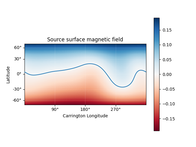
Using the Output object we can plot the source surface field, and the polarity inversion line.

ss_br = pfss_out.source_surface_br
# Create the figure and axes
fig = plt.figure()
ax = plt.subplot(projection=ss_br)

# Plot the source surface map
ss_br.plot()
# Plot the polarity inversion line
ax.plot_coord(pfss_out.source_surface_pils[0])
# Plot formatting
plt.colorbar()
ax.set_title('Source surface magnetic field')

plt.show()

Out:

/home/docs/checkouts/readthedocs.org/user_builds/pfsspy/envs/1.1.1/lib/python3.8/site-packages/pfsspy/output.py:95: UserWarning: Could not parse unit string "Mx/cm^2" as a valid FITS unit.
See https://fits.gsfc.nasa.gov/fits_standard.html for the FITS unit standards.
  warnings.warn(f'Could not parse unit string "{unit_str}" as a valid FITS unit.\n'
INFO: Missing metadata for solar radius: assuming the standard radius of the photosphere. [sunpy.map.mapbase]
/home/docs/checkouts/readthedocs.org/user_builds/pfsspy/envs/1.1.1/lib/python3.8/site-packages/sunpy/map/mapbase.py:590: SunpyMetadataWarning: Missing metadata for observer: assuming Earth-based observer.

  obs_coord = self.observer_coordinate
/home/docs/checkouts/readthedocs.org/user_builds/pfsspy/envs/1.1.1/lib/python3.8/site-packages/pfsspy/output.py:95: UserWarning: Could not parse unit string "Mx/cm^2" as a valid FITS unit.
See https://fits.gsfc.nasa.gov/fits_standard.html for the FITS unit standards.
  warnings.warn(f'Could not parse unit string "{unit_str}" as a valid FITS unit.\n'