Note
Go to the end to download the full example code
GONG PFSS extrapolation
Calculating PFSS solution for a GONG synoptic magnetic field map.
import astropy.constants as const
import astropy.units as u
import matplotlib.pyplot as plt
import numpy as np
import sunpy.map
from astropy.coordinates import SkyCoord

import pfsspy
from pfsspy import coords, tracing
from pfsspy.sample_data import get_gong_map
Load a GONG magnetic field map
gong_fname = get_gong_map()
gong_map = sunpy.map.Map(gong_fname)
The PFSS solution is calculated on a regular 3D grid in (phi, s, rho), where rho = ln(r), and r is the standard spherical radial coordinate. We need to define the number of rho grid points, and the source surface radius.
nrho = 35
rss = 2.5
From the boundary condition, number of radial grid points, and source surface, we now construct an Input object that stores this information
pfss_in = pfsspy.Input(gong_map, nrho, rss)


def set_axes_lims(ax):
    ax.set_xlim(0, 360)
    ax.set_ylim(0, 180)
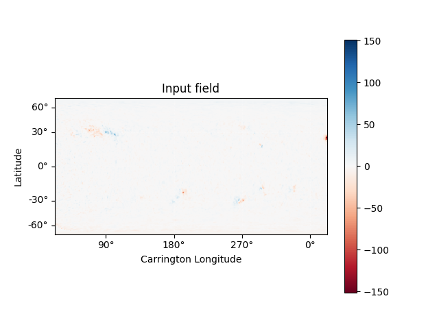
Using the Input object, plot the input field
m = pfss_in.map
fig = plt.figure()
ax = plt.subplot(projection=m)
m.plot()
plt.colorbar()
ax.set_title('Input field')
set_axes_lims(ax)
INFO: Missing metadata for solar radius: assuming the standard radius of the photosphere. [sunpy.map.mapbase]
INFO: Missing metadata for solar radius: assuming the standard radius of the photosphere. [sunpy.map.mapbase]
Now calculate the PFSS solution
pfss_out = pfsspy.pfss(pfss_in)
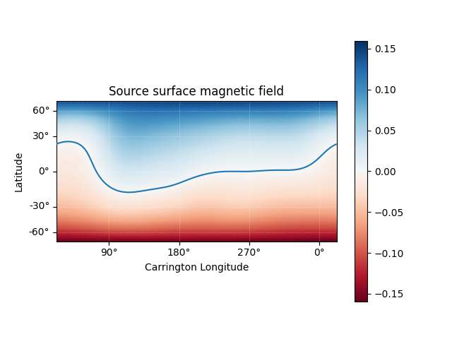
Using the Output object we can plot the source surface field, and the polarity inversion line.
ss_br = pfss_out.source_surface_br
# Create the figure and axes
fig = plt.figure()
ax = plt.subplot(projection=ss_br)

# Plot the source surface map
ss_br.plot()
# Plot the polarity inversion line
ax.plot_coord(pfss_out.source_surface_pils[0])
# Plot formatting
plt.colorbar()
ax.set_title('Source surface magnetic field')
set_axes_lims(ax)
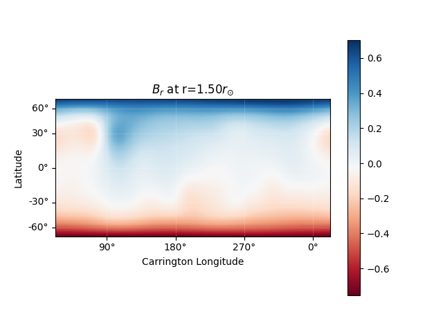
It is also easy to plot the magnetic field at an arbitrary height within the PFSS solution.
# Get the radial magnetic field at a given height
ridx = 15
br = pfss_out.bc[0][:, :, ridx]
# Create a sunpy Map object using output WCS
br = sunpy.map.Map(br.T, pfss_out.source_surface_br.wcs)
# Get the radial coordinate
r = np.exp(pfss_out.grid.rc[ridx])

# Create the figure and axes
fig = plt.figure()
ax = plt.subplot(projection=br)

# Plot the source surface map
br.plot(cmap='RdBu')
# Plot formatting
plt.colorbar()
ax.set_title('$B_{r}$ ' + f'at r={r:.2f}' + '$r_{\\odot}$')
set_axes_lims(ax)
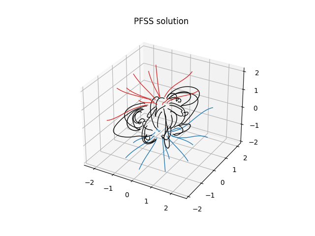
Finally, using the 3D magnetic field solution we can trace some field lines. In this case 64 points equally gridded in theta and phi are chosen and traced from the source surface outwards.
fig = plt.figure()
ax = fig.add_subplot(111, projection='3d')

tracer = tracing.FortranTracer()
r = 1.2 * const.R_sun
lat = np.linspace(-np.pi / 2, np.pi / 2, 8, endpoint=False)
lon = np.linspace(0, 2 * np.pi, 8, endpoint=False)
lat, lon = np.meshgrid(lat, lon, indexing='ij')
lat, lon = lat.ravel() * u.rad, lon.ravel() * u.rad

seeds = SkyCoord(lon, lat, r, frame=pfss_out.coordinate_frame)

field_lines = tracer.trace(seeds, pfss_out)

for field_line in field_lines:
    color = {0: 'black', -1: 'tab:blue', 1: 'tab:red'}.get(field_line.polarity)
    coords = field_line.coords
    coords.representation_type = 'cartesian'
    ax.plot(coords.x / const.R_sun,
            coords.y / const.R_sun,
            coords.z / const.R_sun,
            color=color, linewidth=1)

ax.set_title('PFSS solution')
plt.show()

# sphinx_gallery_thumbnail_number = 4
/home/docs/checkouts/readthedocs.org/user_builds/pfsspy/envs/latest/lib/python3.10/site-packages/pfsspy/tracing.py:180: UserWarning: At least one field line ran out of steps during tracing.
You should probably increase max_steps (currently set to auto) and try again.
  warnings.warn(
Total running time of the script: (0 minutes 7.976 seconds)