Note
Go to the end to download the full example code
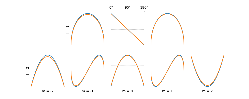
Spherical harmonic comparisons
Comparing analytical spherical harmonic solutions to PFSS output.
import matplotlib.pyplot as plt
import matplotlib.ticker as mticker

from helpers import LMAxes, brss_analytic, brss_pfsspy
Compare the the pfsspy solution to the analytic solutions. Cuts are taken on the source surface at a constant phi value to do a 1D comparison.
nphi = 360
ns = 180
rss = 2
nrho = 20

nl = 2
axs = LMAxes(nl=nl)

for l in range(1, nl+1):
    for m in range(-l, l+1):
        print(f'l={l}, m={m}')
        ax = axs[l, m]

        br_pfsspy = brss_pfsspy(nphi, ns, nrho, rss, l, m)
        br_actual = brss_analytic(nphi, ns, rss, l, m)

        ax.plot(br_pfsspy[:, 15], label='pfsspy')
        ax.plot(br_actual[:, 15], label='analytic')
        if l == 1 and m == 0:
            ax.xaxis.set_major_formatter(mticker.StrMethodFormatter('{x}°'))
            ax.xaxis.set_ticks([0, 90, 180])
            ax.xaxis.tick_top()
            ax.spines['top'].set_visible(True)
        ax.set_xlim(0, 180)
        ax.axhline(0, linestyle='--', linewidth=0.5, color='black')


plt.show()
l=1, m=-1
l=1, m=0
l=1, m=1
l=2, m=-2
l=2, m=-1
l=2, m=0
l=2, m=1
l=2, m=2
Total running time of the script: (0 minutes 21.419 seconds)