Note
Go to the end to download the full example code
Open/closed field map
Creating an open/closed field map on the solar surface.
import astropy.constants as const
import astropy.units as u
import matplotlib.colors as mcolor
import matplotlib.pyplot as plt
import numpy as np
import sunpy.map
from astropy.coordinates import SkyCoord

import pfsspy
from pfsspy import tracing
from pfsspy.sample_data import get_gong_map
Load a GONG magnetic field map
gong_fname = get_gong_map()
gong_map = sunpy.map.Map(gong_fname)
Set the model parameters
nrho = 40
rss = 2.5
Construct the input, and calculate the output solution
pfss_in = pfsspy.Input(gong_map, nrho, rss)
pfss_out = pfsspy.pfss(pfss_in)
Finally, using the 3D magnetic field solution we can trace some field lines. In this case a grid of 90 x 180 points equally gridded in theta and phi are chosen and traced from the source surface outwards.
First, set up the tracing seeds
r = const.R_sun
# Number of steps in cos(latitude)
nsteps = 45
lon_1d = np.linspace(0, 2 * np.pi, nsteps * 2 + 1)
lat_1d = np.arcsin(np.linspace(-1, 1, nsteps + 1))
lon, lat = np.meshgrid(lon_1d, lat_1d, indexing='ij')
lon, lat = lon*u.rad, lat*u.rad
seeds = SkyCoord(lon.ravel(), lat.ravel(), r, frame=pfss_out.coordinate_frame)
INFO: Missing metadata for solar radius: assuming the standard radius of the photosphere. [sunpy.map.mapbase]
INFO: Missing metadata for solar radius: assuming the standard radius of the photosphere. [sunpy.map.mapbase]
Trace the field lines
print('Tracing field lines...')
tracer = tracing.FortranTracer(max_steps=2000)
field_lines = tracer.trace(seeds, pfss_out)
print('Finished tracing field lines')
Tracing field lines...
/home/docs/checkouts/readthedocs.org/user_builds/pfsspy/envs/stable/lib/python3.10/site-packages/pfsspy/tracing.py:180: UserWarning: At least one field line ran out of steps during tracing.
You should probably increase max_steps (currently set to 2000) and try again.
  warnings.warn(
Finished tracing field lines
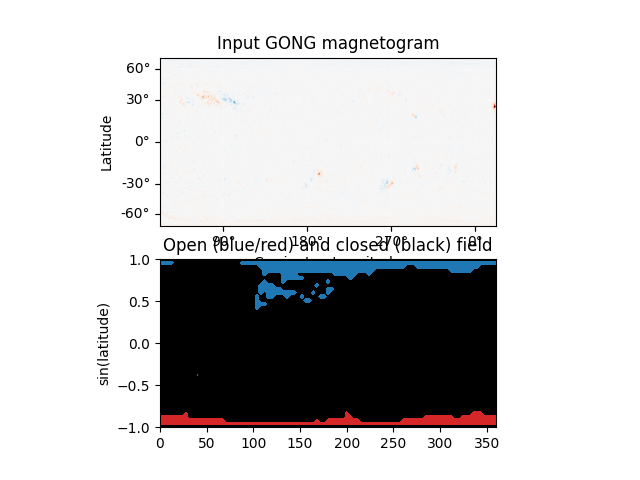
Plot the result. The to plot is the input magnetogram, and the bottom plot shows a contour map of the the footpoint polarities, which are +/- 1 for open field regions and 0 for closed field regions.
fig = plt.figure()
m = pfss_in.map
ax = fig.add_subplot(2, 1, 1, projection=m)
m.plot()
ax.set_title('Input GONG magnetogram')

ax = fig.add_subplot(2, 1, 2)
cmap = mcolor.ListedColormap(['tab:red', 'black', 'tab:blue'])
norm = mcolor.BoundaryNorm([-1.5, -0.5, 0.5, 1.5], ncolors=3)
pols = field_lines.polarities.reshape(2 * nsteps + 1, nsteps + 1).T
ax.contourf(np.rad2deg(lon_1d), np.sin(lat_1d), pols, norm=norm, cmap=cmap)
ax.set_ylabel('sin(latitude)')

ax.set_title('Open (blue/red) and closed (black) field')
ax.set_aspect(0.5 * 360 / 2)

plt.show()
Total running time of the script: (0 minutes 10.459 seconds)