Dipole source solution

A simple example showing how to use pfsspy to compute the solution to a dipole source field.

First, import required modules

import astropy.constants as const
import matplotlib.pyplot as plt
import matplotlib.patches as mpatch
import numpy as np
import pfsspy
import pfsspy.coords as coords

To start with we need to construct an input for the PFSS model. To do this, first set up a regular 2D grid in (phi, s), where s = cos(theta) and (phi, theta) are the standard spherical coordinate system angular coordinates. In this case the resolution is (360 x 180).

nphi = 360
ns = 180

phi = np.linspace(0, 2 * np.pi, nphi)
s = np.linspace(-1, 1, ns)
s, phi = np.meshgrid(s, phi)

Now we can take the grid and calculate the boundary condition magnetic field.

def dipole_Br(r, s):
    return 2 * s / r**3


br = dipole_Br(1, s).T

The PFSS solution is calculated on a regular 3D grid in (phi, s, rho), where rho = ln(r), and r is the standard spherical radial coordinate. We need to define the number of rho grid points, and the source surface radius.

nrho = 50
rss = 2.5

From the boundary condition, number of radial grid points, and source surface, we now construct an Input object that stores this information

input = pfsspy.Input(br, nrho, rss)

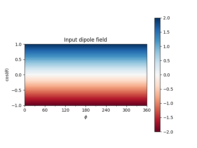
Using the Input object, plot the input field

fig, ax = plt.subplots()
mesh = input.plot_input(ax)
fig.colorbar(mesh)
ax.set_title('Input dipole field')

Now calculate the PFSS solution.

output = pfsspy.pfss(input)

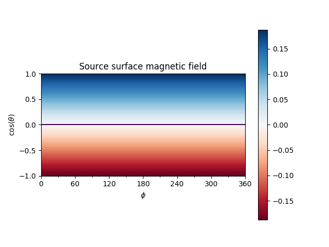
Using the Output object we can plot the source surface field, and the polarity inversion line.

fig, ax = plt.subplots()
mesh = output.plot_source_surface(ax)
fig.colorbar(mesh)
output.plot_pil(ax)
ax.set_title('Source surface magnetic field')

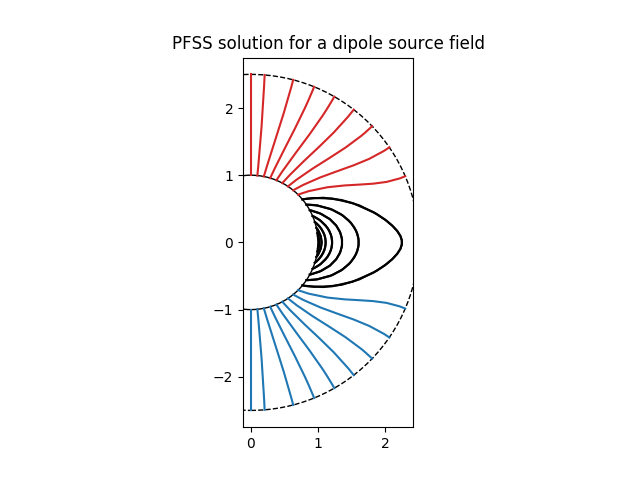
Finally, using the 3D magnetic field solution we can trace some field lines. In this case 32 points equally spaced in theta are chosen and traced from the source surface outwards.

fig, ax = plt.subplots()
ax.set_aspect('equal')

# Take 32 start points spaced equally in theta
r = 1.01
phi = np.pi / 2
for theta in np.linspace(0, np.pi, 33):
    x0 = coords.sph2cart(r, theta, phi)
    field_line = output.trace(np.array(x0))
    color = {0: 'black', -1: 'tab:blue', 1: 'tab:red'}.get(field_line.polarity)
    ax.plot(field_line.y / const.R_sun,
            field_line.z / const.R_sun, color=color)

# Add inner and outer boundary circles
ax.add_patch(mpatch.Circle((0, 0), 1, color='k', fill=False))
ax.add_patch(mpatch.Circle((0, 0), input.grid.rss, color='k', linestyle='--',
                           fill=False))
ax.set_title('PFSS solution for a dipole source field')
plt.show()