GONG PFSS extrapolation

Calculating PFSS solution for a GONG synoptic magnetic field map.

First, import required modules

import os
import astropy.constants as const
import matplotlib.pyplot as plt
from mpl_toolkits.mplot3d import Axes3D
import numpy as np
import sunpy.map

import pfsspy
from pfsspy import coords
from pfsspy import tracing

Load a GONG magnetic field map. If ‘gong.fits’ is present in the current directory, just use that, otherwise download a sample GONG map.

if not os.path.exists('190310t0014gong.fits') and not os.path.exists('190310t0014gong.fits.gz'):
    import urllib.request
    urllib.request.urlretrieve(
        'https://gong2.nso.edu/oQR/zqs/201903/mrzqs190310/mrzqs190310t0014c2215_333.fits.gz',
        '190310t0014gong.fits.gz')

if not os.path.exists('190310t0014gong.fits'):
    import gzip
    with gzip.open('190310t0014gong.fits.gz', 'rb') as f:
        with open('190310t0014gong.fits', 'wb') as g:
            g.write(f.read())

We can now use SunPy to load the GONG fits file, and extract the magnetic field data.

The mean is subtracted to enforce div(B) = 0 on the solar surface: n.b. it is not obvious this is the correct way to do this, so use the following lines at your own risk!

[[br, header]] = sunpy.io.fits.read('190310t0014gong.fits')
br = br - np.mean(br)

GONG maps have their LH edge at -180deg in Carrington Longitude, so roll to get it at 0deg. This way the input magnetic field is in a Carrington frame of reference, which matters later when lining the field lines up with the AIA image.

br = np.roll(br, header['CRVAL1'] + 180, axis=1)

The PFSS solution is calculated on a regular 3D grid in (phi, s, rho), where rho = ln(r), and r is the standard spherical radial coordinate. We need to define the number of rho grid points, and the source surface radius.

nrho = 35
rss = 2.5

From the boundary condition, number of radial grid points, and source surface, we now construct an Input object that stores this information

input = pfsspy.Input(br, nrho, rss)

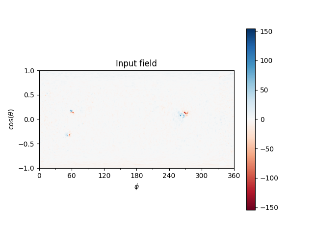
Using the Input object, plot the input field

fig, ax = plt.subplots()
mesh = input.plot_input(ax)
fig.colorbar(mesh)
ax.set_title('Input field')

Out:

Text(0.5, 1.0, 'Input field')

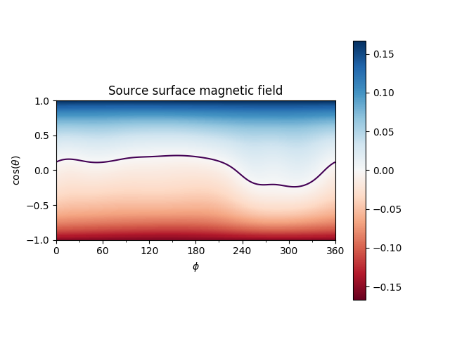
Now calculate the PFSS solution, and plot the polarity inversion line.

output = pfsspy.pfss(input)
output.plot_pil(ax)

Using the Output object we can plot the source surface field, and the polarity inversion line.

fig, ax = plt.subplots()
mesh = output.plot_source_surface(ax)
fig.colorbar(mesh)
output.plot_pil(ax)
ax.set_title('Source surface magnetic field')

Out:

Text(0.5, 1.0, 'Source surface magnetic field')

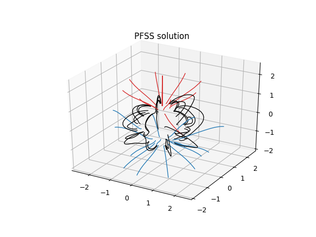
Finally, using the 3D magnetic field solution we can trace some field lines. In this case 64 points equally gridded in theta and phi are chosen and traced from the source surface outwards.

fig = plt.figure()
ax = fig.add_subplot(111, projection='3d')

tracer = tracing.PythonTracer()
r = 1.2
theta = np.linspace(0, np.pi, 8, endpoint=False)
phi = np.linspace(0, 2 * np.pi, 8, endpoint=False)
theta, phi = np.meshgrid(theta, phi)
theta, phi = theta.ravel(), phi.ravel()

seeds = np.array(coords.sph2cart(r, theta, phi)).T

field_lines = tracer.trace(seeds, output)

for field_line in field_lines:
    color = {0: 'black', -1: 'tab:blue', 1: 'tab:red'}.get(field_line.polarity)
    ax.plot(field_line.coords.x / const.R_sun,
            field_line.coords.y / const.R_sun,
            field_line.coords.z / const.R_sun,
            color=color, linewidth=1)

ax.set_title('PFSS solution')
plt.show()

# sphinx_gallery_thumbnail_number = 3