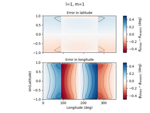
Analytic dipole field lines

First, import required modules

import astropy.constants as const
import astropy.units as u
import matplotlib.pyplot as plt
import numpy as np
from astropy.coordinates import SkyCoord
from astropy.visualization import quantity_support
from helpers import pffspy_output, phi_fline_coords, theta_fline_coords

from pfsspy import tracing

quantity_support()

Out:

<astropy.visualization.units.quantity_support.<locals>.MplQuantityConverter object at 0x7f5d8b26f5d0>

Compare the the pfsspy solution to the analytic solutions. Cuts are taken on the source surface at a constant phi value to do a 1D comparison.

l = 1
m = 1
nphi = 360
ns = 180
nr = 40
rss = 2

Calculate PFSS solution

pfsspy_out = pffspy_output(nphi, ns, nr, rss, l, m)

rss = rss * const.R_sun

Trace some field lines

n = 90
# Create 1D theta, phi arrays
phi = np.linspace(0, 360, n * 2)
phi = phi[:-1] + np.diff(phi) / 2
theta = np.arcsin(np.linspace(-1, 1, n, endpoint=False) + 1/n)
# Mesh into 2D arrays
theta, phi = np.meshgrid(theta, phi, indexing='ij')
theta, phi = theta * u.rad, phi * u.deg
seeds = SkyCoord(radius=rss, lat=theta.ravel(), lon=phi.ravel(),
                 frame=pfsspy_out.coordinate_frame)

step_size = 1
dthetas = []
print(f'Tracing {step_size}...')
# Trace
tracer = tracing.FortranTracer(step_size=step_size)
flines = tracer.trace(seeds, pfsspy_out)
# Set a mask of open field lines
mask = flines.connectivities.astype(bool).reshape(theta.shape)

# Get solar surface latitude
phi_solar = np.ones_like(phi) * np.nan
phi_solar[mask] = flines.open_field_lines.solar_feet.lon
theta_solar = np.ones_like(theta) * np.nan
theta_solar[mask] = flines.open_field_lines.solar_feet.lat
r_out = np.ones_like(theta.value) * const.R_sun * np.nan
r_out[mask] = flines.open_field_lines.solar_feet.radius

Out:

Tracing 1...

Calculate analytical solution

theta_analytic = theta_fline_coords(r_out, rss, l, m, theta)
dtheta = theta_solar - theta_analytic
phi_analytic = phi_fline_coords(r_out, rss, l, m, theta, phi)
dphi = phi_solar - phi_analytic

fig, axs = plt.subplots(nrows=2, sharex=True, sharey=True)


def plot_map(field, ax, label, title):
    kwargs = dict(cmap='RdBu', vmin=-0.5, vmax=0.5, shading='nearest', edgecolors='face')
    im = ax.pcolormesh(phi.to_value(u.deg), np.sin(theta).value,
                       field, **kwargs)
    ax.contour(phi.to_value(u.deg), np.sin(theta).value,
               field,
               levels=[-0.4, -0.3, -0.2, -0.1, 0.1, 0.2, 0.3, 0.4],
               colors='black', alpha=0.5, linewidths=1)
    ax.set_aspect(360 / 4)
    fig.colorbar(im, aspect=10, ax=ax,
                 label=label)
    ax.set_title(title, size=10)


plot_map(dtheta.to_value(u.deg), axs[0],
         r'$\theta_{pfsspy} - \theta_{analytic}$ (deg)',
         'Error in latitude')
plot_map(dphi.to_value(u.deg), axs[1],
         r'$\phi_{pfsspy} - \phi_{analytic}$ (deg)',
         'Error in longitude')

ax = axs[1]
ax.set_xlim(0, 360)
ax.set_ylim(-1, 1)
ax.set_xlabel('Longitude (deg)')
ax.set_ylabel('sin(Latitude)')

fig.suptitle(f'l={l}, m={m}')
fig.tight_layout()
fig.savefig('error_map.pdf', bbox_inches='tight')

plt.show()